Project 13: Customer Retention using Survival Analysis

In this post, I will not be exploring original work - this is not something I modeled independently. I followed this excellent medium tutorial. I am writing this up in order to explore this work a little bit more before applying these techniques to a different dataset. I encourage you to read his post as it has some great explanations and code. The author explains that typically, Customer Churn models are modeled as a binary classification problem defined at some arbitrary threshold. For example, the structuring of the target may look like:

• 0: did not churn in 30 days
• 1: churned in 30 days

This does not have any information on exactly when a customer might churn. Knowing when a customer has a high lapse risk could be very helpful with implementing interventions and contacting the customer at the right time. Survival Analysis is a useful tool for this type of modeling.

Survival Analysis models 'the expected duration of time until an event occurs' ( this page for more information). The author picks up a churn dataset representing customers at a large telecomms company. Our definition of 'lifetime' in the context of this problem is days until lapse. An important concept is that of 'censoring'. This is when the survival time is not known exactly. In our example, this would be for customers who have not churned. Customers who have already churned we have a lifetime for; however, customers who have not yet churned may do so in the future - we don't know. Therefore they are right censored. Another important concept is the survival function. This function describes the probability that a customer will remain longer than time t.

If you would like to follow along, the notebook can be located on my Github or in the tutorial referenced above. An example of what our churn dataset looks like is shown below. There are 20 features including the target, which is we change into a binary representation from a boolean. We are working with 5000 rows (or customers).

churn_df.sample(2)

Since we have almost an exactly event split in the target (churned/didn't churn), the churn rate is close to 50% at 49.96%. We have a feature called 'duration', this is the recorded time in days since opening the account. For customers who churned, this will be equivalent to days until churn. This is important in our modeling, since we want to look at probability of churn over time.

In [9]:

churn_df['duration'].hist(bins=25)

Out[9]:

<AxesSubplot:>

Survival (population-level)

The author first estimates the total survival function for all the customers (the population). This looks something like the cell output below. In order to estimate the survival function, the Kaplan Meier Estimator is used. The Kaplan-Meier survival curve is defined as "the probability of surviving in a given length of time while considering time in many small intervals" (as described here) Or the probability that life is longer than t as described in wikipedia This assumes all customers have the same prospects for survival - regardless if they joined recently or not and whether they lapsed or not.

with:

• ti: the time that event occured
• di: the number of events that happened at time ti
• ni: the individuals known to have survived up to time ti

In [11]:

# estimating the survival function (time in days until attrition)

# Kaplan Meier Estimator is a non-parametric statistic used to estimate the survival function from lifetime data 

kmf = KaplanMeierFitter()

kmf.fit(churn_df['duration'], event_observed=churn_df['event'])

kmf.plot_survival_function()
_=plt.title('Survival Function for Telco Churn');
_=plt.xlabel("Duration: Account Length (days)")
_=plt.ylabel("Churn Risk (Percent Churned)")
_=plt.axvline(x=kmf.median_survival_time_, color='r', linestyle='--')

The red dotted line indicates the median survival time. By this point - 152 days - half the customers have churned. When we implement interventions, we will be able to compare the survival of different groups.

Cox's Proportional Hazard

In order to extract more individual risks on a customer-level, as well as to understand what happens to risk over time (given covariates), the author uses Cox's proportional hazard regression analysis. The hazard rate is the instantaneous probability of event at a given time t, conditional on already having survived that long. It can be thought of as the probability density of event at time t divided by Survival at time t. (for more in-depth information, check out a medium article on this topic ). This article explains why the semi-parametric Cox Proportional Hazards model is popular and useful. To put it into one sentence, it is because it does not need to assume anything about the functional form of the hazard function. Incorrect assumptions about the parametric form of the Hazard function could lead to incorrect conclusions from the model. The Cox Proportional Hazards model only makes assumptions about the effects of the covariates. It allows us to model the effect of multiple risk factors (covariates) on the rate of the event happening at a particular point in time. This is essentially a multiple regression model. It is the linear regression of the log hazard on xi with interpcept = baseline hazard.

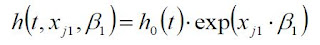
here, the variables are described as follows:

• t: time
• h(t): hazard function determined by a set of p covariates (\(x_1\),...,\(x_p\))
• (\(\beta\)_1,...,\(\beta\)_p): coefficients to be estimated - measure the size of effect of covariates
• \(h_0\): baseline hazard. Corresponds to the value of the hazard if all the xi == 0.

There are a number of good resources detailing this model (firstly this, this, and this are examples). Not to get too lost in the weeds, I will briefly summarize what this model is measuring and a little about its assumptions. The purpose of the model is to evaluate the effect of several factors on survival. This is the rate of a particular event happening at a particular point in time and this rate is commonly referred to as the hazard rate. The quantities \(e^{\beta_i}\) are called the hazard ratios (HR). The \(\beta\) parameters can be interpreted in a similar way to a regression. Taking the case of a single covariate, a \(\beta_{1}\) value of 0.1 indicates that increasing the covariate by an amount of 1 leads to an approximately \(10\%\) increase in the event occurence at any given time (\(10\%\) increase in the hazard rate). A negative beta indicates a decrease in risk and beta=0 means no effect.

The Cox model assumes that hazard ratios or relative risks remain constant over time. For different levels within a covariate, their hazard ratios do not depend on time. If different covariates have disproportionate hazards, stratification can be used. Similarly, if different groups within the data have different risks at different times.

Modeling

The author of the original medium post we are working through describes the transformation of the target. Target is duration - positive for occurence of event, negative for 'non-events' (no churn). We can use XGBoost in order to learn the parameter set. The objective involves a partial likelihood. This was proposed by Cox in order to estimate the beta parameters without needings \(\lambda_{0}(t)\) (baseline hazard.) I'll use the term 'failure' to denote event (in our case churn) since this is the accepted way of referring to it. The partial likelihood is calculated is the conditional probability of an observed individual being chosen from the risk set to fail. The risk set denotes the set of individuals who are 'at risk' of failure at time t. In the XGBoost model, we set the 'objective' to 'survival:cox' and the rest of the parameters as usual. We can look at the predictions as the Hazard Ratio (exponentiated).

In [37]:

_=df_test.groupby(pd.qcut(df_test['duration'], q=20))['preds_exp'].median().plot(kind="bar")

Evaluation

The author of the post uses Harrell's Concordance Index and Brier Score. Harrell's C-index is commonly used to evaluate risk models and provide a goodness of fit measure. It measures concordance between any two individuals in the population where the pair is concordant if the risk is higher for the individual with failure at a shorter time and discordant if otherwise. The measure takes into account censoring of individuals. It can simply be described as \(\frac{\textrm{num concordant pairs}}{\textrm{num concordant pairs} + \textrm{number discordant pairs}}\).

Therefore, values near 0.5 show that the risk score predictions are no better than a coin toss in determining churn times. Values near one indicate that the risk score is very good at determining which of two customers might churn first. Values near zero are worse than a coin flip and you might be better off concluding the opposite of what the risk score tells you. (Here is an excellent blog post explaining)

The time dependent Brier score is an extension of the mean squared error to right censored data and is only applicable to models which estimate a survival function. If a model predicts 10% risk of experiencing an event at a time \(t\), the observed frequency in the data should support this for a well-calibrated model. The error the Brier Score measures is between the observed survival status (churned/ not churned: 1/0) and the predicted survival probability (a number between 0 and 1). When the data contains right-censoring, the score is adjusted by weighting the sqaured distances using the inverse probability of censoring weights method [1] A Brier Score of 1/3 is as good as random chance, 0 is a perfect score and a score towards 1 is not great.

_, y_train = get_x_y(df_train,['event','duration'],pos_label=True)
_, y_test = get_x_y(df_test,['event','duration'],pos_label=True)

del _

print("CIC")
print(
    surv_metrics.concordance_index_ipcw(
       y_train,
       y_test,
      df_test['preds'],
        tau=100 # within 100 days
    )
)

print("")
print("Brier Score")

times, score = surv_metrics.brier_score(
y_train,y_test, df_test['preds'], df_test['duration'].max() - 1
)
print(score)

CIC
(0.7280474978540299, 187246, 70953, 0, 1288)

Brier Score
[0.85096896]

What I really like is how the author does a bit of model explainability. The SHAP plots allow us to understand how different factors influence attrition or churn.

In [39]:

explainer = shap.TreeExplainer(bst, feature_names=feature_names)
shap_values = explainer.shap_values(test_features) 

shap.summary_plot(shap_values, pd.DataFrame(test_features, columns=feature_names))

From our summary SHAP plot, we can see that high day_mins increase attrition, while low day_mins decrease it. Very intuitively, high night_charges increase attrition while low night charges decrease it, and so on. These are the factors we can start to look into optimizing for the customers. At a customer level, we can look at a SHAP force plot (below). The random customer we chose seems to have churned, and the largest three contributing factors were day_mins, night_calls and night_mins.

In [40]:

idx_sample = 128
shap.force_plot(
    explainer.expected_value,
    shap_values[idx_sample, :],
    pd.DataFrame(test_features, columns=feature_names).iloc[idx_sample, :],
    matplotlib=True,
)

print(f"The real label is Churn={y_test[idx_sample][0]}")

The real label is Churn=True

I learned a lot working through this. I had never done survivial analysis before, but I can see how it can be used in a host of applications and I'm excited to test some more things out.

[1] https://square.github.io/pysurvival/metrics/brier_score.html